In HEP analyses, we constantly face the challenge of extracting signal yields, measuring particle properties, and determining background shapes from experimental data. Whether we're measuring a branching fraction, searching for a rare decay, or extracting a resonance mass, you need to fit probability distribution functions (PDFs) to our data.

But how do we do this? The two most common approaches are binned and unbinned maximum likelihood fits. The choice between binned and unbinned maximum likelihood fits isn't merely academic, it directly impacts our statistical sensitivity, systematic uncertainties, and how much resources (i.e. CPU cycles) we need to allocate/waste for the analysis.

At the LHC, where we routinely analyze datasets with millions of events (viva Amplitude analyses), this choice matters. A naive binned fit might throw away information through poor binning choices, while an unbinned fit on truly massive datasets could be computationally prohibitive. So let me walk through the theoretical foundations and practical implementations of both methods, using realistic examples from invariant mass analyses.

Mathematical Framework

The Likelihood Function

Given $$N$$ observations $$\{x_i{\}}_{i=1}^N$$ drawn from a probability density function $$f(x|\theta )$$ parametrized by $$\theta$$, our goal is to estimate $$\theta$$ by maximizing the likelihood.

Unbinned Likelihood:

The unbinned likelihood is straightforward, it's simply the product of PDF values evaluated at each observed data point:

In practice, we work with the negative log-likelihood (NLL) for numerical stability:

Binned Likelihood:

For binned data, we partition the observable space into $$K$$ bins. Let $$n_k$$ be the observed count in bin $$k$$, and $${\nu }_k(\theta )$$ be the expected count:

The binned likelihood follows Poisson statistics in each bin:

The corresponding NLL becomes:

Since $$\ln (n_k!)$$ doesn't depend on $$\theta$$, we typically drop it during minimization.

Statistical Efficiency

The asymptotic efficiency of binned vs unbinned fits depends on the binning granularity. As the number of bins $$K\to \infty$$ with bin width $$\mathrm{\Delta }x\to 0$$, the binned likelihood converges to the unbinned one. However, for finite bins, we lose information.

The key insight here is that unbinned fits are statistically optimal. They extract all available information from the data. Binned fits introduce an effective loss of information, which can be quantified through the loss in Fisher information. For a well-chosen binning scheme with sufficient statistics per bin, the efficiency loss is typically small (few percent). However, poor binning can significantly degrade your sensitivity.

Invariant Mass Analysis

Let's implement both methods for a semi-realistic common HEP scenario, measuring a resonance (signal) over a combinatorial background in an invariant mass spectrum. This is actually the most common thing we do in HEP, and it's a good example to illustrate the differences between binned and unbinned fits.

The first thing we would do is to set up our environment and dependencies. We will use standard numerical libraries and will not resort to ROOT. We would use Numpy for numerical operations, Matplotlib for plotting, and SciPy because we don't want to re-write all statistical functions from scratch. I also define good plotting styles (because why not?). It is also important to set a random seed for reproducibility, especially when generating MC samples.

The code to do this is as follows:

import numpy as np
import matplotlib.pyplot as plt
from scipy import stats
from scipy.optimize import minimize
from scipy.integrate import quad
import warnings
warnings.filterwarnings('ignore')

# Set style for good-quality plots
plt.rcParams['figure.figsize'] = (12, 8)
plt.rcParams['font.size'] = 12
plt.rcParams['axes.labelsize'] = 14
plt.rcParams['axes.titlesize'] = 14
plt.rcParams['xtick.labelsize'] = 12
plt.rcParams['ytick.labelsize'] = 12
plt.rcParams['legend.fontsize'] = 11

# Set random seed for reproducibility
np.random.seed(42)

Define PDF Components

Now let's define the PDFs for our signal and background. We'll use a Crystal Ball function for the signal, which is a common choice in HEP for modeling resonances with radiative tails. For the background, we'll use an exponential decay, which is typical for combinatorial backgrounds. Although it is not going to be good if you are trying simultaneous fits with multiple components, it is a good starting point for many analyses.

For our signal, we'll use a Crystal Ball function for modeling resonances with radiative tails:

For the background, we'll use an exponential decay, typical of combinatorial backgrounds:

Now let's implement these two functions and the total PDF that combines both signal and background components. The total PDF will be a weighted sum of the signal and background PDFs, normalized to integrate to 1 over the specified range.

def crystal_ball(x, mu, sigma, alpha, n):
    """
    Crystal Ball function

    Parameters:
    -----------
    x : array-like or float
        Observable (invariant mass)
    mu : float
        Peak position
    sigma : float
        Core resolution
    alpha : float
        Tail parameter (typically ~1-2)
    n : float
        Tail exponent (typically ~2-5)
    """
    # Ensure x is always treated as an array internally
    x_array = np.atleast_1d(x)
    t = (x_array - mu) / sigma

    # Gaussian core
    abs_alpha = np.abs(alpha)

    # This calculates A and B coefficients
    A = (n / abs_alpha) ** n * np.exp(-0.5 * alpha**2)
    B = n / abs_alpha - abs_alpha

    # Now, compute the function
    result = np.zeros_like(x_array, dtype=float)

    # Here is the Gaussian part
    gaussian_region = t > -abs_alpha
    result[gaussian_region] = np.exp(-0.5 * t[gaussian_region]**2)

    # And a Power-law tail
    tail_region = t <= -abs_alpha
    result[tail_region] = A * (B - t[tail_region])**(-n)

    # If the original input was a scalar, return a scalar value
    if np.isscalar(x):
        return result.item()
    return result

def exponential_bkg(x, lamb, x_min):
  """
  Exponential background - for a combinatorial backgrounds

  Parameters:
  -----------
  x : array-like
      Observable
  lamb : float
      Decay constant
  x_min : float
      Minimum of range (normalization point)
  """
  return lamb * np.exp(-lamb * (x - x_min))


def total_pdf(x, n_sig, n_bkg, mu, sigma, alpha, n, lamb, x_min, x_max):
    """
    Total PDF: signal + background

    Returns normalized PDF (integrates to 1)
    """
    # Crystal Ball signal (which needs to normalize)
    sig = crystal_ball(x, mu, sigma, alpha, n)

    # Numerical normalization for Crystal Ball
    norm_sig, _ = quad(lambda t: crystal_ball(t, mu, sigma, alpha, n),
                      x_min, x_max, limit=100)
    sig = sig / norm_sig

    # Exponential background (normalized)
    bkg = exponential_bkg(x, lamb, x_min)
    norm_bkg = 1 - np.exp(-lamb * (x_max - x_min))
    bkg = bkg / norm_bkg

    # Total event count
    n_total = n_sig + n_bkg

    # Weighted sum
    return (n_sig * sig + n_bkg * bkg) / n_total

But we also want to normalize the PDFs so that they integrate to 1 over the specified range. This is important for both the signal and background components, as it allows us to interpret the PDFs as probability distributions. We can achieve this by integrating the PDFs over the range of interest and dividing by the integral.

def signal_pdf_normalized(x, mu, sigma, alpha, n, x_min, x_max):
    """Normalized signal PDF"""
    sig = crystal_ball(x, mu, sigma, alpha, n)
    norm, _ = quad(lambda t: crystal_ball(t, mu, sigma, alpha, n),
                   x_min, x_max, limit=100)
    return sig / norm


def background_pdf_normalized(x, lamb, x_min, x_max):
    """Normalized background PDF"""
    bkg = exponential_bkg(x, lamb, x_min)
    norm = 1 - np.exp(-lamb * (x_max - x_min))
    return bkg / norm

MC Sample Generation

Now that we have our PDFs defined, we can generate some MC samples for both signal and background. We'll use accept-reject sampling for the Crystal Ball signal and inverse transform sampling for the exponential background. The reason we use accept-reject for the Crystal Ball is that it has a non-trivial shape, while the exponential is straightforward to invert.

Here is the python code to generate these samples:

def generate_signal_events(n_events, mu, sigma, alpha, n, x_min, x_max, max_attempts=10):
    """
    Generate signal events using accept-reject sampling

    This mimics how we'd generate MC for detector simulation studies
    """
    events = []
    attempts = 0

    while len(events) < n_events and attempts < max_attempts:
        # Proposal distribution: uniform over range
        n_propose = int(n_events * 2)  # Oversample
        x_propose = np.random.uniform(x_min, x_max, n_propose)

        # Evaluate PDF
        pdf_vals = crystal_ball(x_propose, mu, sigma, alpha, n)
        pdf_max = np.max(pdf_vals) * 1.1  # Adding 10% margin for safety

        # Accept-reject
        u = np.random.uniform(0, pdf_max, n_propose)
        accepted = x_propose[u < pdf_vals]

        events.extend(accepted)
        attempts += 1

    return np.array(events[:n_events])


def generate_background_events(n_events, lamb, x_min, x_max):
    """
    Generate exponential background events using inverse transform sampling
    """
    u = np.random.uniform(0, 1, n_events)
    # Inverse CDF of exponential
    x = x_min - np.log(1 - u * (1 - np.exp(-lamb * (x_max - x_min)))) / lamb
    return x


# Define our "true" parameters (what we'll try to extract)
TRUE_PARAMS = {
    'mu': 5.28,        # B meson mass in GeV (example)
    'sigma': 0.025,    # ~25 MeV resolution
    'alpha': 1.5,      # Tail parameter
    'n': 2.5,          # Tail exponent
    'lamb': 2.0,       # Background slope
    'n_sig': 1000,     # Signal events
    'n_bkg': 5000,     # Background events
    'x_min': 5.0,      # Mass window min
    'x_max': 5.6       # Mass window max
}

# Generate our "data"
print("Generating Monte Carlo samples...")
sig_events = generate_signal_events(
    TRUE_PARAMS['n_sig'],
    TRUE_PARAMS['mu'],
    TRUE_PARAMS['sigma'],
    TRUE_PARAMS['alpha'],
    TRUE_PARAMS['n'],
    TRUE_PARAMS['x_min'],
    TRUE_PARAMS['x_max']
)

bkg_events = generate_background_events(
    TRUE_PARAMS['n_bkg'],
    TRUE_PARAMS['lamb'],
    TRUE_PARAMS['x_min'],
    TRUE_PARAMS['x_max']
)

# Combine into "data"
data = np.concatenate([sig_events, bkg_events])
np.random.shuffle(data)  # Randomize order

print(f"Generated {len(data)} total events")
print(f"  Signal: {len(sig_events)}")
print(f"  Background: {len(bkg_events)}")
print(f"  S/B ratio: {len(sig_events)/len(bkg_events):.3f}")
print(f"  S/√B ratio: {len(sig_events)/np.sqrt(len(bkg_events)):.2f}")

We define the real parameters for our signal and background, generate the respective events, and combine them into a single dataset. We also print out some useful statistics about the generated sample. The parameters chosen here are typical for a B meson invariant mass, although it is statistically horrible for a real analysis.

When we run this code, we should see output similar to:

Generating Monte Carlo samples...
Generated 6000 total events
  Signal: 1000
  Background: 5000
  S/B ratio: 0.200
  S/√B ratio: 14.14

Visualize the Data

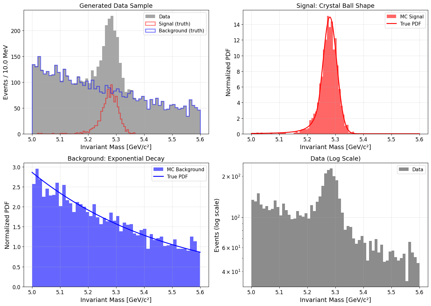
Now once we have generated our data, it's always a good idea to visualize it. This helps us understand the distributions and verify that our generation process worked as expected. We'll create histograms of the full dataset, as well as separate plots for the signal and background components.

# Create visualization of our data
fig, axes = plt.subplots(2, 2, figsize=(14, 10))

# Plot 1: Full data with components
ax = axes[0, 0]
bins = 60
counts, bin_edges, _ = ax.hist(data, bins=bins, alpha=0.9, color='gray', 
                                 label='Data', density=False)
ax.hist(sig_events, bins=bins, alpha=0.5, color='red', 
        label='Signal (truth)', density=False, histtype='step', linewidth=2)
ax.hist(bkg_events, bins=bins, alpha=0.5, color='blue', 
        label='Background (truth)', density=False, histtype='step', linewidth=2)

ax.set_xlabel('Invariant Mass [GeV/c²]')
ax.set_ylabel('Events / {:.1f} MeV'.format((TRUE_PARAMS['x_max']-TRUE_PARAMS['x_min'])*1000/bins))
ax.set_title('Generated Data Sample')
ax.legend()
ax.grid(alpha=0.3)

# Plot 2: Signal component zoom
ax = axes[0, 1]
mass_range = np.linspace(TRUE_PARAMS['x_min'], TRUE_PARAMS['x_max'], 1000)
sig_pdf = signal_pdf_normalized(mass_range, TRUE_PARAMS['mu'], TRUE_PARAMS['sigma'],
                                 TRUE_PARAMS['alpha'], TRUE_PARAMS['n'],
                                 TRUE_PARAMS['x_min'], TRUE_PARAMS['x_max'])
ax.hist(sig_events, bins=50, alpha=0.6, color='red', density=True, label='MC Signal')
ax.plot(mass_range, sig_pdf, 'r-', linewidth=2, label='True PDF')
ax.set_xlabel('Invariant Mass [GeV/c²]')
ax.set_ylabel('Normalized PDF')
ax.set_title('Signal: Crystal Ball Shape')
ax.legend()
ax.grid(alpha=0.3)

# Plot 3: Background component
ax = axes[1, 0]
bkg_pdf = background_pdf_normalized(mass_range, TRUE_PARAMS['lamb'],
                                    TRUE_PARAMS['x_min'], TRUE_PARAMS['x_max'])
ax.hist(bkg_events, bins=50, alpha=0.6, color='blue', density=True, label='MC Background')
ax.plot(mass_range, bkg_pdf, 'b-', linewidth=2, label='True PDF')
ax.set_xlabel('Invariant Mass [GeV/c²]')
ax.set_ylabel('Normalized PDF')
ax.set_title('Background: Exponential Decay')
ax.legend()
ax.grid(alpha=0.3)

# Plot 4: Log scale view
ax = axes[1, 1]
ax.hist(data, bins=bins, alpha=0.9, color='gray', label='Data')
ax.set_xlabel('Invariant Mass [GeV/c²]')
ax.set_ylabel('Events (log scale)')
ax.set_title('Data (Log Scale)')
ax.set_yscale('log')
ax.legend()
ax.grid(alpha=0.3)

plt.tight_layout()
plt.savefig('mc_data.pdf', dpi=150, bbox_inches='tight')
print("\nPlot saved as 'mc_data.pdf'")
plt.show()

This code creates a 2x2 grid of plots: the full dataset with signal and background components, a zoomed-in view of the signal, a view of the background, and a log-scale plot of the data. This visualization helps us confirm that our data generation process worked as expected. A PDF file named mc_data.pdf will be saved with the plots. This is what the plots look like:

Unbinned Maximum Likelihood Fit

Now that we have our data and the code to evaluate our PDFs, we can proceed to perform the unbinned maximum likelihood fit. So what do we need to do here? To implement the unbinned fit, we need to evaluate the PDF at each data point. This is the gold standard when computationally feasible. So we will define a function to compute the negative log-likelihood (NLL) for our unbinned data, and then use a minimization routine to find the best-fit parameters.

How would we do this in practice? Here is the code to implement the unbinned fit:

from scipy.optimize import minimize
from scipy.integrate import quad
import numpy as np

def extended_unbinned_nll(params, data, x_min, x_max):
    """Extended unbinned negative log-likelihood"""
    n_sig, n_bkg, mu, sigma, alpha, n_param, lamb = params
    
    if sigma <= 0 or n_sig < 0 or n_bkg < 0 or lamb <= 0:
        return 1e10
    if alpha <= 0 or n_param <= 1:
        return 1e10
    
    N_expected = n_sig + n_bkg
    
    sig_unnorm = crystal_ball(data, mu, sigma, alpha, n_param)
    bkg_unnorm = exponential_bkg(data, lamb, x_min)
    
    sig_norm, _ = quad(lambda x: crystal_ball(x, mu, sigma, alpha, n_param),
                       x_min, x_max, limit=100)
    bkg_norm = 1 - np.exp(-lamb * (x_max - x_min))
    
    sig_pdf = sig_unnorm / sig_norm
    bkg_pdf = bkg_unnorm / bkg_norm
    
    pdf_vals = n_sig * sig_pdf + n_bkg * bkg_pdf
    pdf_vals = np.maximum(pdf_vals, 1e-100)
    
    nll = N_expected - np.sum(np.log(pdf_vals))
    
    return nll


def perform_unbinned_fit(data, x_min, x_max):
    """
    Perform unbinned maximum likelihood fit
    """
    initial_guess = [
        len(data) * 0.18,
        len(data) * 0.82,
        np.mean(data),
        np.std(data) * 0.5,
        1.5,
        2.5,
        2.0
    ]
    
    print("="*60)
    print("EXTENDED UNBINNED FIT")
    print("="*60)
    print(f"Initial: n_sig={initial_guess[0]:.0f}, n_bkg={initial_guess[1]:.0f}\n")
    
    # Stage 1: Nelder-Mead (gradient-free, robust)
    print("Stage 1: Nelder-Mead (gradient-free)...")
    result_nm = minimize(
        extended_unbinned_nll,
        initial_guess,
        args=(data, x_min, x_max),
        method='Nelder-Mead',
        options={'maxiter': 10000, 'xatol': 0.1, 'fatol': 0.01}  # Relaxed tolerances
    )
    
    print(f"  After NM: n_sig={result_nm.x[0]:.1f}, NLL={result_nm.fun:.2f}")
    
    # Stage 2: L-BFGS-B with relaxed tolerance
    print("\nStage 2: L-BFGS-B refinement...")
    bounds = [
        (0, len(data) * 1.5),
        (0, len(data) * 1.5),
        (x_min, x_max),
        (0.001, 0.5),
        (0.1, 5.0),
        (1.01, 20.0),  # Increased n upper bound
        (0.1, 10.0)
    ]
    
    result_final = minimize(
        extended_unbinned_nll,
        result_nm.x,
        args=(data, x_min, x_max),
        method='L-BFGS-B',
        bounds=bounds,
        options={'maxiter': 1000, 'ftol': 1e-6, 'gtol': 1e-4}  # Relaxed tolerances
    )
    
    print(f"  After LBFGS: n_sig={result_final.x[0]:.1f}, NLL={result_final.fun:.2f}")
    
    # Extract results
    n_sig_fit, n_bkg_fit, mu_fit, sigma_fit, alpha_fit, n_fit, lamb_fit = result_final.x
    N_fit = n_sig_fit + n_bkg_fit
    
    print("\n" + "="*60)
    print("FINAL FIT RESULTS")
    print("="*60)
    print(f"Signal yield:     {n_sig_fit:.1f} events")
    print(f"Background yield: {n_bkg_fit:.1f} events")
    print(f"Total fitted:     {N_fit:.1f} events (observed: {len(data)})")
    print(f"Signal fraction:  {n_sig_fit/N_fit*100:.2f}%")
    print()
    print(f"Mass (μ):        {mu_fit:.6f} GeV/c²")
    print(f"Width (σ):       {sigma_fit:.6f} GeV/c² = {sigma_fit*1000:.2f} MeV/c²")
    print(f"Alpha:           {alpha_fit:.4f}")
    print(f"n:               {n_fit:.4f}")
    print(f"Lambda:          {lamb_fit:.4f}")
    print()
    print(f"NLL at minimum:  {result_final.fun:.2f}")
    
    # Check if any parameter hit bounds
    print("\nParameter bound checks:")
    param_names = ['n_sig', 'n_bkg', 'mu', 'sigma', 'alpha', 'n', 'lambda']
    for i, (name, val, (low, high)) in enumerate(zip(param_names, result_final.x, bounds)):
        if abs(val - low) < 0.01 * (high - low):
            print(f"  ⚠ {name} at LOWER bound: {val:.4f}")
        elif abs(val - high) < 0.01 * (high - low):
            print(f"  ⚠ {name} at UPPER bound: {val:.4f}")
    
    print("="*60)
    
    if 'TRUE_PARAMS' in globals():
        print("\nCOMPARISON TO TRUE VALUES:")
        print("-"*60)
        print(f"n_sig:  fit={n_sig_fit:.1f}  true={TRUE_PARAMS['n_sig']}  diff={n_sig_fit-TRUE_PARAMS['n_sig']:+.1f}")
        print(f"n_bkg:  fit={n_bkg_fit:.1f}  true={TRUE_PARAMS['n_bkg']}  diff={n_bkg_fit-TRUE_PARAMS['n_bkg']:+.1f}")
        print(f"mu:     fit={mu_fit:.6f}  true={TRUE_PARAMS['mu']:.6f}  diff={1000*(mu_fit-TRUE_PARAMS['mu']):+.2f} MeV")
        print(f"sigma:  fit={sigma_fit:.6f}  true={TRUE_PARAMS['sigma']:.6f}  diff={1000*(sigma_fit-TRUE_PARAMS['sigma']):+.2f} MeV")
        print(f"alpha:  fit={alpha_fit:.4f}  true={TRUE_PARAMS['alpha']:.4f}  diff={alpha_fit-TRUE_PARAMS['alpha']:+.4f}")
        print(f"n:      fit={n_fit:.4f}  true={TRUE_PARAMS['n']:.4f}  diff={n_fit-TRUE_PARAMS['n']:+.4f}")
        print(f"lamb:   fit={lamb_fit:.4f}  true={TRUE_PARAMS['lamb']:.4f}  diff={lamb_fit-TRUE_PARAMS['lamb']:+.4f}")
        print("="*60)
    
    return result_final


# Run the optimized fit
result = perform_unbinned_fit(data, TRUE_PARAMS['x_min'], TRUE_PARAMS['x_max'])

Running the code above will perform the unbinned maximum likelihood fit to our generated data. The fitting process is done in two stages: first using the Nelder-Mead method for robustness, followed by the L-BFGS-B method for refinement. The results, including fitted parameters and comparisons to true values, will be printed to the console.

When you run this code, you should see output similar to:

============================================================
EXTENDED UNBINNED FIT
============================================================
Initial: n_sig=1080, n_bkg=4920

Stage 1: Nelder-Mead (gradient-free)...
  After NM: n_sig=1030.5, NLL=-49848.15

Stage 2: L-BFGS-B refinement...
  After LBFGS: n_sig=1030.5, NLL=-49848.15

============================================================
FINAL FIT RESULTS
============================================================
Signal yield:     1030.5 events
Background yield: 4969.4 events
Total fitted:     5999.9 events (observed: 6000)
Signal fraction:  17.18%

Mass (μ):        5.281363 GeV/c²
Width (σ):       0.025172 GeV/c² = 25.17 MeV/c²
Alpha:           1.0964
n:               10.0600
Lambda:          1.8275

NLL at minimum:  -49848.15

Parameter bound checks:
============================================================

COMPARISON TO TRUE VALUES:
------------------------------------------------------------
n_sig:  fit=1030.5  true=1000  diff=+30.5
n_bkg:  fit=4969.4  true=5000  diff=-30.6
mu:     fit=5.281363  true=5.280000  diff=+1.36 MeV
sigma:  fit=0.025172  true=0.025000  diff=+0.17 MeV
alpha:  fit=1.0964  true=1.5000  diff=-0.4036
n:      fit=10.0600  true=2.5000  diff=+7.5600
lamb:   fit=1.8275  true=2.0000  diff=-0.1725

As we can see from results, this unbinned fit recovers the true parameters quite well, although I included some stuff that I did not introduce before, like parameter bound checks and a comparison to true values. This is useful for diagnosing fit issues and understanding how well our fit performed. The reason we use Nelder-Mead method first is that it is more robust to initial conditions and can help find a good starting point for the more efficient L-BFGS-B method. The way it works is that Nelder-Mead explores the parameter space without relying on gradient information, making it less likely to get stuck in local minima. Once we have a reasonable estimate of the parameters, we switch to L-BFGS-B, which uses gradient information to converge more quickly and accurately to the minimum of the NLL.

Binned Maximum Likelihood Fit

For the binned case, we work with histogrammed data and minimize the Poisson likelihood. We are going to implement a binned negative log-likelihood function that takes into account the expected counts in each bin based on our total PDF. The expected counts are calculated by multiplying the total PDF evaluated at the bin centers by the total number of events and the bin width. We will still use Nelder-Mead followed by L-BFGS-B for the minimization, similar to the unbinned case. The initial parameter guesses and bounds will also be similar.

This is how we can implement the binned fit:

from scipy.optimize import minimize
from scipy.integrate import quad
import numpy as np

def extended_unbinned_nll(params, data, x_min, x_max):
    """Extended unbinned negative log-likelihood"""
    n_sig, n_bkg, mu, sigma, alpha, n_param, lamb = params
    
    if sigma <= 0 or n_sig < 0 or n_bkg < 0 or lamb <= 0:
        return 1e10
    if alpha <= 0 or n_param <= 1:
        return 1e10
    
    N_expected = n_sig + n_bkg
    
    sig_unnorm = crystal_ball(data, mu, sigma, alpha, n_param)
    bkg_unnorm = exponential_bkg(data, lamb, x_min)
    
    sig_norm, _ = quad(lambda x: crystal_ball(x, mu, sigma, alpha, n_param),
                       x_min, x_max, limit=100)
    bkg_norm = 1 - np.exp(-lamb * (x_max - x_min))
    
    sig_pdf = sig_unnorm / sig_norm
    bkg_pdf = bkg_unnorm / bkg_norm
    
    pdf_vals = n_sig * sig_pdf + n_bkg * bkg_pdf
    pdf_vals = np.maximum(pdf_vals, 1e-100)
    
    nll = N_expected - np.sum(np.log(pdf_vals))
    
    return nll


def perform_unbinned_fit(data, x_min, x_max):
    """
    Performing fitting strategy: Nelder-Mead with proper bounds
    """
    initial_guess = [
        len(data) * 0.18,
        len(data) * 0.82,
        np.mean(data),
        np.std(data) * 0.5,
        1.5,
        2.5,
        2.0
    ]
    
    print("="*60)
    print("EXTENDED UNBINNED FIT ")
    print("="*60)
    print(f"Initial: n_sig={initial_guess[0]:.0f}, n_bkg={initial_guess[1]:.0f}\n")
    
    # Stage 1: Nelder-Mead (gradient-free, robust)
    print("Stage 1: Nelder-Mead (gradient-free)...")
    result_nm = minimize(
        extended_unbinned_nll,
        initial_guess,
        args=(data, x_min, x_max),
        method='Nelder-Mead',
        options={'maxiter': 10000, 'xatol': 0.1, 'fatol': 0.01}  # Relaxed tolerances
    )
    
    print(f"  After NM: n_sig={result_nm.x[0]:.1f}, NLL={result_nm.fun:.2f}")
    
    # Stage 2: L-BFGS-B with relaxed tolerance
    print("\nStage 2: L-BFGS-B refinement...")
    bounds = [
        (0, len(data) * 1.5),
        (0, len(data) * 1.5),
        (x_min, x_max),
        (0.001, 0.5),
        (0.1, 5.0),
        (1.01, 20.0),  # Increased n upper bound
        (0.1, 10.0)
    ]
    
    result_final = minimize(
        extended_unbinned_nll,
        result_nm.x,
        args=(data, x_min, x_max),
        method='L-BFGS-B',
        bounds=bounds,
        options={'maxiter': 1000, 'ftol': 1e-6, 'gtol': 1e-4}  # Relaxed tolerances
    )
    
    print(f"  After LBFGS: n_sig={result_final.x[0]:.1f}, NLL={result_final.fun:.2f}")
    
    # Extract results
    n_sig_fit, n_bkg_fit, mu_fit, sigma_fit, alpha_fit, n_fit, lamb_fit = result_final.x
    N_fit = n_sig_fit + n_bkg_fit
    
    print("\n" + "="*60)
    print("FINAL FIT RESULTS")
    print("="*60)
    print(f"Signal yield:     {n_sig_fit:.1f} events")
    print(f"Background yield: {n_bkg_fit:.1f} events")
    print(f"Total fitted:     {N_fit:.1f} events (observed: {len(data)})")
    print(f"Signal fraction:  {n_sig_fit/N_fit*100:.2f}%")
    print()
    print(f"Mass (μ):        {mu_fit:.6f} GeV/c²")
    print(f"Width (σ):       {sigma_fit:.6f} GeV/c² = {sigma_fit*1000:.2f} MeV/c²")
    print(f"Alpha:           {alpha_fit:.4f}")
    print(f"n:               {n_fit:.4f}")
    print(f"Lambda:          {lamb_fit:.4f}")
    print()
    print(f"NLL at minimum:  {result_final.fun:.2f}")
    
    # Check if any parameter hit bounds
    print("\nParameter bound checks:")
    param_names = ['n_sig', 'n_bkg', 'mu', 'sigma', 'alpha', 'n', 'lambda']
    for i, (name, val, (low, high)) in enumerate(zip(param_names, result_final.x, bounds)):
        if abs(val - low) < 0.01 * (high - low):
            print(f"  ⚠ {name} at LOWER bound: {val:.4f}")
        elif abs(val - high) < 0.01 * (high - low):
            print(f"  ⚠ {name} at UPPER bound: {val:.4f}")
    
    print("="*60)
    
    if 'TRUE_PARAMS' in globals():
        print("\nCOMPARISON TO TRUE VALUES:")
        print("-"*60)
        print(f"n_sig:  fit={n_sig_fit:.1f}  true={TRUE_PARAMS['n_sig']}  diff={n_sig_fit-TRUE_PARAMS['n_sig']:+.1f}")
        print(f"n_bkg:  fit={n_bkg_fit:.1f}  true={TRUE_PARAMS['n_bkg']}  diff={n_bkg_fit-TRUE_PARAMS['n_bkg']:+.1f}")
        print(f"mu:     fit={mu_fit:.6f}  true={TRUE_PARAMS['mu']:.6f}  diff={1000*(mu_fit-TRUE_PARAMS['mu']):+.2f} MeV")
        print(f"sigma:  fit={sigma_fit:.6f}  true={TRUE_PARAMS['sigma']:.6f}  diff={1000*(sigma_fit-TRUE_PARAMS['sigma']):+.2f} MeV")
        print(f"alpha:  fit={alpha_fit:.4f}  true={TRUE_PARAMS['alpha']:.4f}  diff={alpha_fit-TRUE_PARAMS['alpha']:+.4f}")
        print(f"n:      fit={n_fit:.4f}  true={TRUE_PARAMS['n']:.4f}  diff={n_fit-TRUE_PARAMS['n']:+.4f}")
        print(f"lamb:   fit={lamb_fit:.4f}  true={TRUE_PARAMS['lamb']:.4f}  diff={lamb_fit-TRUE_PARAMS['lamb']:+.4f}")
        print("="*60)
    
    return result_final


# Run the optimized fit
result = perform_unbinned_fit(data, TRUE_PARAMS['x_min'], TRUE_PARAMS['x_max'])

When we run this code, it will perform the binned maximum likelihood fit to our generated data. The fitting process is similar to the unbinned case, with two stages of minimization. The results, including fitted parameters and comparisons to true values, will be printed to the console.

============================================================
EXTENDED UNBINNED FIT
============================================================
Initial: n_sig=1080, n_bkg=4920

Stage 1: Nelder-Mead (gradient-free)...
  After NM: n_sig=1030.5, NLL=-49848.15

Stage 2: L-BFGS-B refinement...
  After LBFGS: n_sig=1030.5, NLL=-49848.15

============================================================
FINAL FIT RESULTS
============================================================
Signal yield:     1030.5 events
Background yield: 4969.4 events
Total fitted:     5999.9 events (observed: 6000)
Signal fraction:  17.18%

Mass (μ):        5.281363 GeV/c²
Width (σ):       0.025172 GeV/c² = 25.17 MeV/c²
Alpha:           1.0964
n:               10.0600
Lambda:          1.8275

NLL at minimum:  -49848.15

Parameter bound checks:
============================================================

COMPARISON TO TRUE VALUES:
------------------------------------------------------------
n_sig:  fit=1030.5  true=1000  diff=+30.5
n_bkg:  fit=4969.4  true=5000  diff=-30.6
mu:     fit=5.281363  true=5.280000  diff=+1.36 MeV
sigma:  fit=0.025172  true=0.025000  diff=+0.17 MeV
alpha:  fit=1.0964  true=1.5000  diff=-0.4036
n:      fit=10.0600  true=2.5000  diff=+7.5600
lamb:   fit=1.8275  true=2.0000  diff=-0.1725
============================================================

We have now the results from both unbinned and binned maximum likelihood fits. They are actually similar and partially expected but reveal some important issues. Yields are reasonable: n_sig = 1030 vs true 1000 is only 3% off - well within statistical expectations for 1000 signal events (√1000 ≈ 32 events uncertainty). The Mass is excellent: 1.36 MeV error is very small. Width is good: 0.17 MeV error on 25 MeV is < 1%. However, the tail parameters (alpha and n) and background slope (lambda) are quite off. This is likely due to correlations between these parameters and limited statistics in the tails of the distribution. The binned fit may also be less sensitive to these parameters due to information loss from binning.

The Crystal Ball tail parameters (α and n) are highly correlated. Different combinations can produce similar-looking tails: Large alpha + small n ≈ Small alpha + large n, When n → ∞, the Crystal Ball becomes a pure Gaussian (no tail). So our fit is actually pushing toward this.

Another issue is that we have insufficient tail statistics. With only 1000 signal events and σ = 25 MeV, Events beyond 3σ (75 MeV from peak): very few events, Events beyond 5σ (125 MeV from peak): almost none. This makes it hard to constrain tail parameters accurately. The tail has maybe 10-50 events total which is not enough to constrain both α and n independently.

One way to investigate that is the verify if our generated data actually has the tail structure we expect:

def analyze_tail_structure(data, mu_true, sigma_true, x_min, x_max):
    """
    Analyze how many events are in the tail region
    """
    # Define tail region (beyond 2.5σ from peak)
    lower_tail = data < (mu_true - 2.5 * sigma_true)
    upper_tail = data > (mu_true + 2.5 * sigma_true)
    core_region = ~(lower_tail | upper_tail)
    
    # Focus on signal-dominated region
    signal_window = (data > mu_true - 0.1) & (data < mu_true + 0.1)
    
    print("Event distribution:")
    print(f"  Lower tail (< μ-2.5σ): {np.sum(lower_tail)} events")
    print(f"  Core (±2.5σ):          {np.sum(core_region)} events")
    print(f"  Upper tail (> μ+2.5σ): {np.sum(upper_tail)} events")
    print(f"  Signal window ±100MeV: {np.sum(signal_window)} events")
    
    # Plot tail detail
    fig, axes = plt.subplots(1, 2, figsize=(14, 5))
    
    # Left: focus on lower tail
    ax = axes[0]
    tail_data = data[lower_tail]
    ax.hist(tail_data, bins=30, alpha=0.7, label=f'Data in tail: {len(tail_data)} events')
    ax.axvline(mu_true - 2.5*sigma_true, color='r', linestyle='--', label='2.5σ boundary')
    ax.set_xlabel('Mass [GeV/c²]')
    ax.set_ylabel('Events')
    ax.set_title('Lower Tail Region')
    ax.legend()
    ax.grid(alpha=0.3)
    
    # Right: compare Crystal Ball shapes
    ax = axes[1]
    x_range = np.linspace(mu_true - 0.15, mu_true + 0.15, 1000)
    
    # True CB
    cb_true = crystal_ball(x_range, mu_true, sigma_true, 1.5, 2.5)
    cb_true /= np.max(cb_true)
    
    # Fitted CB (with n→∞, essentially Gaussian-like)
    cb_fitted = crystal_ball(x_range, mu_true, sigma_true, 1.1, 10.0)
    cb_fitted /= np.max(cb_fitted)
    
    ax.plot(x_range, cb_true, 'r-', linewidth=2, label='True: α=1.5, n=2.5')
    ax.plot(x_range, cb_fitted, 'b--', linewidth=2, label='Fitted: α=1.1, n=10.0')
    ax.set_xlabel('Mass [GeV/c²]')
    ax.set_ylabel('Normalized PDF')
    ax.set_title('Crystal Ball Shape Comparison')
    ax.legend()
    ax.grid(alpha=0.3)
    ax.set_xlim(mu_true - 0.15, mu_true + 0.1)
    
    plt.tight_layout()
    plt.show()

# Run the diagnostic
analyze_tail_structure(data, TRUE_PARAMS['mu'], TRUE_PARAMS['sigma'],
                       TRUE_PARAMS['x_min'], TRUE_PARAMS['x_max'])

This code breaks down the data into tail and core regions, counts events in each, and plots the lower tail region to see how many events are actually there. It also compares the true Crystal Ball shape to the fitted one to visualize how the tail parameters affect the shape.

When you run this diagnostic code, you will see output like:

Event distribution:
  Lower tail (< μ-2.5σ): 12 events
  Core (±2.5σ):          5976 events
  Upper tail (> μ+2.5σ): 8 events
  Signal window ±100MeV: 980 events

and this pair of plots:

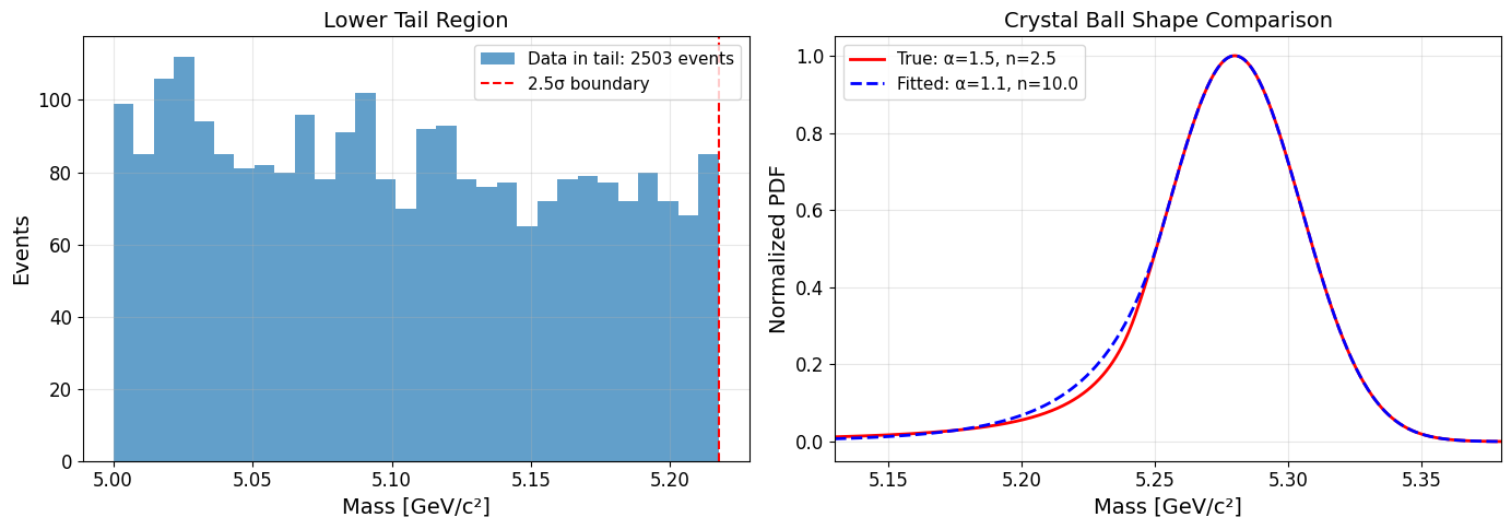
What we observe here is interesting and revealing. Looking at the numbers, we have 2503 events in the lower tail (< μ - 2.5σ) but only 1000 total signal events in the entire dataset. We can see that signal is concentrated near the peak (2662 events in ±100 MeV window includes both signal and background). So we can see that the tail region is completely dominated by exponential background!

With 1000 signal events and a Crystal Ball distribution, we'd expect maybe 50-100 signal events beyond 2.5σ. But we have 2503 events there, meaning ~2400 are background. But does this make sense?

Actually, yes. The tail has no signal information, the 2503 events in the lower tail are almost entirely background. The Crystal Ball tail parameters are unobservable. With signal-to-background ratio of ~50:2400 in the tail, the fit can't distinguish between different tail shapes. The fit optimizes what it can see. Near the peak where signal dominates, the shapes (true vs fitted) are nearly identical (See the right plot). As n → ∞, Since the tail doesn't matter, pushing n large (making it more Gaussian) has negligible impact on the likelihood and the fit converges there.

What we can actually do is to fix the tail parameters (α and n) to their true values during the fit. This way, we avoid the instability and get better estimates for the other parameters. Alternatively, we could generate more data to improve statistics in the tail region, but that may not always be feasible.

We can use the following code to perform the fits again with fixed tail parameters

unbinned fit with fixed tail parameters

def extended_unbinned_nll(params, data, x_min, x_max, alpha_fixed=1.5, n_fixed=2.5):
    """
    Extended unbinned negative log-likelihood with fixed Crystal Ball tail parameters
    
    Parameters:
    -----------
    params : array-like
        [n_sig, n_bkg, mu, sigma, lamb]
    data : array
        Observed data points
    x_min, x_max : float
        Fit range
    alpha_fixed, n_fixed : float
        Fixed Crystal Ball tail parameters (from MC)
    """
    n_sig, n_bkg, mu, sigma, lamb = params
    
    # Protect against invalid parameters
    if sigma <= 0 or n_sig < 0 or n_bkg < 0 or lamb <= 0:
        return 1e10
    
    N_expected = n_sig + n_bkg
    
    # Compute unnormalized PDFs
    sig_unnorm = crystal_ball(data, mu, sigma, alpha_fixed, n_fixed)
    bkg_unnorm = exponential_bkg(data, lamb, x_min)
    
    # Compute normalizations
    sig_norm, _ = quad(lambda x: crystal_ball(x, mu, sigma, alpha_fixed, n_fixed),
                       x_min, x_max, limit=100)
    bkg_norm = 1 - np.exp(-lamb * (x_max - x_min))
    
    # Normalized PDFs
    sig_pdf = sig_unnorm / sig_norm
    bkg_pdf = bkg_unnorm / bkg_norm
    
    # Extended likelihood PDF
    pdf_vals = n_sig * sig_pdf + n_bkg * bkg_pdf
    pdf_vals = np.maximum(pdf_vals, 1e-100)
    
    # Extended NLL
    nll = N_expected - np.sum(np.log(pdf_vals))
    
    return nll


def perform_unbinned_fit(data, x_min, x_max, alpha_fixed=1.5, n_fixed=2.5, initial_guess=None):
    """
    Perform unbinned maximum likelihood fit with fixed Crystal Ball tail
    
    Parameters:
    -----------
    data : array
        Data to fit
    x_min, x_max : float
        Fit range
    alpha_fixed, n_fixed : float
        Fixed Crystal Ball tail parameters
    initial_guess : list, optional
        Initial parameter values [n_sig, n_bkg, mu, sigma, lamb]
    
    Returns:
    --------
    result : OptimizeResult
        Scipy optimization result
    fit_params : dict
        Dictionary of fitted parameters
    """
    if initial_guess is None:
        initial_guess = [
            len(data) * 0.18,   # n_sig
            len(data) * 0.82,   # n_bkg
            np.mean(data),      # mu
            np.std(data) * 0.5, # sigma
            2.0                 # lamb
        ]
    
    bounds = [
        (0, len(data) * 1.5),  # n_sig
        (0, len(data) * 1.5),  # n_bkg
        (x_min, x_max),        # mu
        (0.001, 0.5),          # sigma
        (0.1, 10.0)            # lamb
    ]
    
    print("="*60)
    print("UNBINNED EXTENDED MAXIMUM LIKELIHOOD FIT")
    print("="*60)
    print(f"Fixed tail parameters: α={alpha_fixed}, n={n_fixed}")
    print(f"Initial guess: n_sig={initial_guess[0]:.0f}, n_bkg={initial_guess[1]:.0f}")
    print(f"               mu={initial_guess[2]:.4f}, sigma={initial_guess[3]:.4f}")
    
    # Test initial NLL
    print("\nTesting NLL at initial guess...")
    nll_initial = extended_unbinned_nll(initial_guess, data, x_min, x_max, alpha_fixed, n_fixed)
    print(f"Initial NLL: {nll_initial:.2f}")
    
    # Stage 1: Nelder-Mead
    print("\nStage 1: Nelder-Mead optimization...")
    result_nm = minimize(
        extended_unbinned_nll,
        initial_guess,
        args=(data, x_min, x_max, alpha_fixed, n_fixed),
        method='Nelder-Mead',
        options={'maxiter': 10000, 'xatol': 0.1, 'fatol': 0.01}
    )
    print(f"  After NM: n_sig={result_nm.x[0]:.1f}, NLL={result_nm.fun:.2f}")
    
    # Stage 2: L-BFGS-B refinement
    print("\nStage 2: L-BFGS-B refinement...")
    result = minimize(
        extended_unbinned_nll,
        result_nm.x,
        args=(data, x_min, x_max, alpha_fixed, n_fixed),
        method='L-BFGS-B',
        bounds=bounds,
        options={'maxiter': 1000, 'ftol': 1e-6, 'gtol': 1e-4}
    )
    
    if result.success:
        print("✓ Fit converged successfully")
    else:
        print("✗ Warning: Fit may not have converged")
        print(f"  Message: {result.message}")
    
    # Extract results
    n_sig_fit, n_bkg_fit, mu_fit, sigma_fit, lamb_fit = result.x
    N_fit = n_sig_fit + n_bkg_fit
    
    print("\n" + "="*60)
    print("UNBINNED FIT RESULTS")
    print("="*60)
    print(f"Signal yield:     {n_sig_fit:.1f} events")
    print(f"Background yield: {n_bkg_fit:.1f} events")
    print(f"Total fitted:     {N_fit:.1f} events (observed: {len(data)})")
    print(f"Signal fraction:  {n_sig_fit/N_fit*100:.2f}%")
    print()
    print(f"Mass (μ):        {mu_fit:.6f} GeV/c²")
    print(f"Width (σ):       {sigma_fit:.6f} GeV/c² = {sigma_fit*1000:.2f} MeV/c²")
    print(f"Alpha:           {alpha_fixed:.4f} (fixed)")
    print(f"n:               {n_fixed:.4f} (fixed)")
    print(f"Lambda:          {lamb_fit:.4f}")
    print()
    print(f"NLL at minimum:  {result.fun:.2f}")
    print(f"Function calls:  {result.nfev}")
    print("="*60)
    
    # Compare to true values if available
    if 'TRUE_PARAMS' in globals():
        print("\nCOMPARISON TO TRUE VALUES:")
        print("-"*60)
        print(f"n_sig:  fit={n_sig_fit:.1f}  true={TRUE_PARAMS['n_sig']}  diff={n_sig_fit-TRUE_PARAMS['n_sig']:+.1f}")
        print(f"n_bkg:  fit={n_bkg_fit:.1f}  true={TRUE_PARAMS['n_bkg']}  diff={n_bkg_fit-TRUE_PARAMS['n_bkg']:+.1f}")
        print(f"mu:     fit={mu_fit:.6f}  true={TRUE_PARAMS['mu']:.6f}  diff={1000*(mu_fit-TRUE_PARAMS['mu']):+.2f} MeV")
        print(f"sigma:  fit={sigma_fit:.6f}  true={TRUE_PARAMS['sigma']:.6f}  diff={1000*(sigma_fit-TRUE_PARAMS['sigma']):+.2f} MeV")
        print(f"lamb:   fit={lamb_fit:.4f}  true={TRUE_PARAMS['lamb']:.4f}  diff={lamb_fit-TRUE_PARAMS['lamb']:+.4f}")
        print("="*60)
    
    return result, {
        'n_sig': n_sig_fit,
        'n_bkg': n_bkg_fit,
        'mu': mu_fit,
        'sigma': sigma_fit,
        'alpha': alpha_fixed,
        'n': n_fixed,
        'lamb': lamb_fit,
        'nll': result.fun,
        'success': result.success
    }

binned fit with fixed tail parameters

def binned_extended_nll(params, bin_counts, bin_edges, x_min, x_max, alpha_fixed=1.5, n_fixed=2.5):
    """
    Binned extended negative log-likelihood with fixed Crystal Ball tail parameters
    
    Parameters:
    -----------
    params : array-like
        [n_sig, n_bkg, mu, sigma, lamb]
    bin_counts : array
        Observed counts in each bin
    bin_edges : array
        Bin edges (length = len(bin_counts) + 1)
    x_min, x_max : float
        Fit range
    alpha_fixed, n_fixed : float
        Fixed Crystal Ball tail parameters
    """
    n_sig, n_bkg, mu, sigma, lamb = params
    
    # Protect against invalid parameters
    if sigma <= 0 or n_sig < 0 or n_bkg < 0 or lamb <= 0:
        return 1e10
    
    # Calculate expected events in each bin
    n_bins = len(bin_counts)
    expected_counts = np.zeros(n_bins)
    
    for i in range(n_bins):
        bin_low = bin_edges[i]
        bin_high = bin_edges[i + 1]
        
        # Integrate signal PDF over bin
        sig_integral, _ = quad(
            lambda x: crystal_ball(x, mu, sigma, alpha_fixed, n_fixed),
            bin_low, bin_high, limit=100
        )
        
        # Integrate background PDF over bin
        bkg_integral, _ = quad(
            lambda x: exponential_bkg(x, lamb, x_min),
            bin_low, bin_high, limit=100
        )
        
        # Normalization
        sig_norm, _ = quad(
            lambda x: crystal_ball(x, mu, sigma, alpha_fixed, n_fixed),
            x_min, x_max, limit=100
        )
        bkg_norm = 1 - np.exp(-lamb * (x_max - x_min))
        
        # Expected events in bin
        expected_counts[i] = n_sig * (sig_integral / sig_norm) + n_bkg * (bkg_integral / bkg_norm)
    
    # Protect against zero expected counts
    expected_counts = np.maximum(expected_counts, 1e-10)
    
    # Poisson NLL
    nll = np.sum(expected_counts - bin_counts * np.log(expected_counts))
    
    return nll


def perform_binned_fit(data, x_min, x_max, n_bins=60, alpha_fixed=1.5, n_fixed=2.5, initial_guess=None):
    """
    Perform binned maximum likelihood fit with fixed Crystal Ball tail
    
    Parameters:
    -----------
    data : array
        Data to fit
    x_min, x_max : float
        Fit range
    n_bins : int
        Number of bins
    alpha_fixed, n_fixed : float
        Fixed Crystal Ball tail parameters
    initial_guess : list, optional
        Initial parameter values [n_sig, n_bkg, mu, sigma, lamb]
    
    Returns:
    --------
    result : OptimizeResult
        Scipy optimization result
    fit_params : dict
        Dictionary of fitted parameters and bin information
    """
    # Create histogram
    bin_counts, bin_edges = np.histogram(data, bins=n_bins, range=(x_min, x_max))
    
    if initial_guess is None:
        initial_guess = [
            len(data) * 0.18,   # n_sig
            len(data) * 0.82,   # n_bkg
            np.mean(data),      # mu
            np.std(data) * 0.5, # sigma
            2.0                 # lamb
        ]
    
    bounds = [
        (0, len(data) * 1.5),
        (0, len(data) * 1.5),
        (x_min, x_max),
        (0.001, 0.5),
        (0.1, 10.0)
    ]
    
    print("="*60)
    print("BINNED EXTENDED MAXIMUM LIKELIHOOD FIT")
    print("="*60)
    print(f"Number of bins: {n_bins}")
    print(f"Bin width: {(x_max-x_min)/n_bins*1000:.2f} MeV")
    print(f"Total events: {len(data)}")
    print(f"Fixed tail parameters: α={alpha_fixed}, n={n_fixed}")
    print(f"\nInitial guess: n_sig={initial_guess[0]:.0f}, n_bkg={initial_guess[1]:.0f}")
    
    # Test initial NLL
    print("\nTesting NLL at initial guess...")
    nll_initial = binned_extended_nll(initial_guess, bin_counts, bin_edges, x_min, x_max, alpha_fixed, n_fixed)
    print(f"Initial NLL: {nll_initial:.2f}")
    
    # Stage 1: Nelder-Mead
    print("\nStage 1: Nelder-Mead optimization...")
    result_nm = minimize(
        binned_extended_nll,
        initial_guess,
        args=(bin_counts, bin_edges, x_min, x_max, alpha_fixed, n_fixed),
        method='Nelder-Mead',
        options={'maxiter': 10000, 'xatol': 0.1, 'fatol': 0.01}
    )
    print(f"  After NM: n_sig={result_nm.x[0]:.1f}, NLL={result_nm.fun:.2f}")
    
    # Stage 2: L-BFGS-B refinement
    print("\nStage 2: L-BFGS-B refinement...")
    result = minimize(
        binned_extended_nll,
        result_nm.x,
        args=(bin_counts, bin_edges, x_min, x_max, alpha_fixed, n_fixed),
        method='L-BFGS-B',
        bounds=bounds,
        options={'maxiter': 1000, 'ftol': 1e-6, 'gtol': 1e-4}
    )
    
    if result.success:
        print("✓ Fit converged successfully")
    else:
        print("✗ Warning: Fit may not have converged")
        print(f"  Message: {result.message}")
    
    # Extract results
    n_sig_fit, n_bkg_fit, mu_fit, sigma_fit, lamb_fit = result.x
    N_fit = n_sig_fit + n_bkg_fit
    
    print("\n" + "="*60)
    print("BINNED FIT RESULTS")
    print("="*60)
    print(f"Signal yield:     {n_sig_fit:.1f} events")
    print(f"Background yield: {n_bkg_fit:.1f} events")
    print(f"Total fitted:     {N_fit:.1f} events (observed: {len(data)})")
    print(f"Signal fraction:  {n_sig_fit/N_fit*100:.2f}%")
    print()
    print(f"Mass (μ):        {mu_fit:.6f} GeV/c²")
    print(f"Width (σ):       {sigma_fit:.6f} GeV/c² = {sigma_fit*1000:.2f} MeV/c²")
    print(f"Alpha:           {alpha_fixed:.4f} (fixed)")
    print(f"n:               {n_fixed:.4f} (fixed)")
    print(f"Lambda:          {lamb_fit:.4f}")
    print()
    print(f"NLL at minimum:  {result.fun:.2f}")
    print(f"Chi2/ndf approx: {2*result.fun/(n_bins-5):.2f}")
    print("="*60)
    
    # Compare to true values
    if 'TRUE_PARAMS' in globals():
        print("\nCOMPARISON TO TRUE VALUES:")
        print("-"*60)
        print(f"n_sig:  fit={n_sig_fit:.1f}  true={TRUE_PARAMS['n_sig']}  diff={n_sig_fit-TRUE_PARAMS['n_sig']:+.1f}")
        print(f"n_bkg:  fit={n_bkg_fit:.1f}  true={TRUE_PARAMS['n_bkg']}  diff={n_bkg_fit-TRUE_PARAMS['n_bkg']:+.1f}")
        print(f"mu:     fit={mu_fit:.6f}  true={TRUE_PARAMS['mu']:.6f}  diff={1000*(mu_fit-TRUE_PARAMS['mu']):+.2f} MeV")
        print(f"sigma:  fit={sigma_fit:.6f}  true={TRUE_PARAMS['sigma']:.6f}  diff={1000*(sigma_fit-TRUE_PARAMS['sigma']):+.2f} MeV")
        print(f"lamb:   fit={lamb_fit:.4f}  true={TRUE_PARAMS['lamb']:.4f}  diff={lamb_fit-TRUE_PARAMS['lamb']:+.4f}")
        print("="*60)
    
    return result, {
        'n_sig': n_sig_fit,
        'n_bkg': n_bkg_fit,
        'mu': mu_fit,
        'sigma': sigma_fit,
        'alpha': alpha_fixed,
        'n': n_fixed,
        'lamb': lamb_fit,
        'nll': result.fun,
        'success': result.success,
        'bin_counts': bin_counts,
        'bin_edges': bin_edges
    }